August 12, 2026
World Models From Scratch, Part 2: Frozen Versus Joint
The zero from part 1 becomes 0.81 with a GRU bolted onto a frozen encoder, and 0.96 when the encoder learns from the prediction loss. Along the way: a model with the best one-step error in the experiment that leaves the data manifold by its thirtieth prediction, and an agent trained on nothing but hallucinations.
That is the end goal of this post, running live: the trained weights, executing in your browser. The white ball is steered by the policy this post builds, from those 32x32 pixels and nothing else. Put the goal wherever you like; it was trained on goals that cruise and bounce, so one that teleports under your cursor is a situation it never saw, and it copes.
The strip underneath is the strange part. Nothing renders those frames: from what the model currently believes, it imagines the next 16 steps with no further pixels arriving (training used 15). That imagination was the policy's only training environment: the policy was trained entirely inside this world model, all 5,000 actor updates, and never saw a real transition until it was evaluated.
Part 1 ended with a zero: velocity from the VAE's latent, and no training could have fixed it, because a single frame contains no velocity. This post gives a model 33 frames at once, then does it again a second way, because there are two ways to attach memory to an encoder and the difference between them is the whole point of the series.
1. The frozen recipe: a GRU on a frozen encoder
Result of this block: a GRU trained on the frozen part-1 latents reads velocity at 0.81, and every variant of it has lost the real ball by 20 open-loop steps. The setup is the first six sections; the numbers start at "Results: four GRUs".
The recipe, and the seam
Ha and Schmidhuber's World Models (2018) trains a VAE first, freezes it, and trains a recurrent model on its latents. The defining property of the recipe is not the GRU. It is the seam.
The paper's parts are V, a VAE that compresses frames to latents, M, a recurrent network that predicts the next latent, and C, a tiny controller evolved with CMA-ES. I build V and M and skip C; block 3 replaces it with something better anyway.
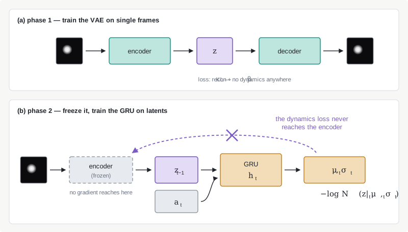
Whatever reconstruction happened to preserve is all the dynamics model will ever get, and however the encoder arranged it is the coordinate system the dynamics model has to work in. Part 1 measured both costs in advance: about 5.4 nats per frame, in a code curled enough that a linear probe reads position at 0.75 rather than the 0.9+ the design doc expected.
Why split at all? Because in 2018 it was the thing that worked: training a big conv encoder jointly with a recurrent model was unstable, and decoupling them turns one hard optimization into two easy ones. What it costs is what block 2 measures.
The model: one GRU cell and a Gaussian head
One GRU cell with 128 hidden units, a small MLP head that emits a Gaussian over the next latent, and a negative log-likelihood (NLL) loss.
The hidden state is 128 and stays 128 for the rest of the post, including the RSSM, so that probes on different models read states of the same dimension. The code and the smaller details are in the box.
The GRU in code, plus the σ floor, the single-Gaussian head, and latent standardization. Open if you are reimplementing, or want the MDN-RNN comparison.
class GRUDynamics(nn.Module):
latent_dim: int = 16
action_dim: int = 2
hidden: int = 128
residual: bool = False
@nn.compact
def __call__(self, h, z_prev, action):
x = jnp.concatenate([z_prev, action], axis=-1)
h, _ = nn.GRUCell(features=self.hidden)(h, x)
y = nn.silu(nn.Dense(128)(h))
mu = nn.Dense(self.latent_dim)(y)
sigma = jax.nn.softplus(nn.Dense(self.latent_dim)(y)) + 1e-3
if self.residual:
mu = z_prev + mu
return h, mu, sigma
- has a floor of . Gaussian NLL is unbounded below: a model that drives on an easy target earns arbitrarily large likelihood and takes the loss with it.
softplus(raw) + 1e-3makes that impossible. Every likelihood-based model in this project has a floor somewhere; it is the cheapest instability insurance there is. - A single Gaussian head. Ha and Schmidhuber use an MDN-RNN, a mixture-density head, which is worth it when the next-latent distribution is multimodal. For a ball in a box it mostly isn't; the one candidate is a wall bounce. I left the MDN as an ablation to run if the single Gaussian visibly underfit at bounces. It didn't, so I didn't.
- Latents are standardized per dimension before the GRU sees them, with mean and std fit on the training episodes and stored in the checkpoint. Part 1 showed nine active dimensions and seven idling near the prior; without standardization the NLL is dominated by whichever dimensions have large variance.
Why a GRU can recover velocity when the encoder cannot
The GRU state is the first object in the pipeline that ever sees a sequence, and the NLL objective forces a velocity estimate into it.
Nothing in the architecture is smarter than the VAE; the GRU cannot see pixels, only the same frozen 16 numbers per frame that scored zero on velocity. But velocity is , a function of two frames, absent from any single one, and is a function of everything up to , so it can hold one.
Whether it will is decided by the loss. The NLL is minimized by predicting the conditional expectation,
and for a ball with momentum that expectation depends on position and velocity. A state that dropped velocity would predict the same next frame for a ball moving left as for one moving right, and pay for it in likelihood at every step of every sequence.
Training setup, and the two switches
Subsequences of 33 frames, teacher forced, with the first four transitions masked out of the loss. Then a 2x2 grid over two design forks that papers usually pick without comment.
Subsequences are sampled uniformly from the training episodes; batch 64, Adam at , 20k steps, one lax.scan over time. 32 transitions contain a couple of bounces (arithmetic in the box), so linear extrapolation will not do.
- , and the first four transitions are excluded from the loss. With no history the velocity is unknowable, so those steps would only teach the model to hedge. The same warm-up of 4 is used at evaluation time, for both models in this post.
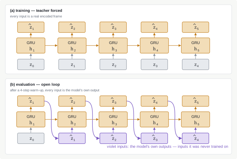
- Training is teacher forced. At every step the GRU receives the true , never its own prediction.
That last one is standard, and it sets up the most useful failure in this post:
Now the switches:
- Direct or residual? Should the head predict , or the change ? Residual is standard wisdom for smooth dynamics, since the change is small and easy to fit.
- Means or samples? The frozen encoder emits . Encode the dataset to posterior means, or to samples?
Instead of choosing, I ran the 2x2, four GRUs identical except for those switches, about 3 GPU-minutes each:
uv run train-gru --predict direct --latent-source mean
uv run train-gru --predict residual --latent-source mean
uv run train-gru --predict direct --latent-source sample
uv run train-gru --predict residual --latent-source sample
Where 33 frames comes from, and why "residual" is a mean offset rather than a density over Δz. Open if you will change the sequence length or compare the NLL column.
The speed cap is 2 pixels per step and the dataset's mean speed is 1.41, so a crossing of the 32-pixel box takes 16 to 23 steps, and 32 transitions contain a couple of bounces.
"Residual" is implemented as a mean offset, , so all four models put a density on the same variable and their likelihoods are comparable. A density over instead would need a change-of-variables term before any NLL column meant anything.
Why a small error becomes a large one
In a world with walls, open-loop error does not grow smoothly. A bounce turns a small disagreement about where into a total disagreement about when.
Give the two balls below a nudge apart and watch what the wall does to it:
ball A vs ball B, started 0.05 px/step apart
distance now 1.90 px
Nothing in that demo is a neural network. It is the environment from part 1, run twice from almost the same state, and it puts a floor under every drift curve in this post: before the first mispredicted bounce, errors grow slowly, and after it the two timelines are unrelated.
How to read a pixel-error curve
The evaluation is an open-loop rollout: warm up on 4 real transitions, run the model forward on its own mean predictions for 30 steps, decode each predicted latent, and measure pixel MSE against the real continuation. That number is drift in every table below. rollout.py implements it once and both models in this post call it.
A pixel MSE of 0.018 means nothing until you know the scale. The reference levels that make every number in this post readable:
| level | per-pixel MSE | meaning |
|---|---|---|
| mean image | ≈ 0.011 | knows nothing, admits it |
| hallucination ceiling (an uncorrelated ball) | ≈ 0.022 | knows nothing, insists otherwise; far above this, the model has left the space of ball images |
| frozen pipeline floor | ≈ 0.00027 | the autoencoding round trip; no GRU prediction can beat it |
The third level is specific to each pipeline rather than to the data, because every GRU prediction is decoded by the frozen decoder from latents produced by the frozen encoder. The RSSM's floor will turn out to be completely different, and the comparison in block 2 is meaningless without both.
Where the three levels come from, and the units trap between part 1's 0.28 and this post's 0.0004. Derivation; skip unless you want to re-derive 0.011 and 0.022.
Mean image. A model that gives up and paints the dataset's mean image has per-pixel error equal to the pixel variance:
Uncorrelated ball. A model that draws a perfectly good ball in an uncorrelated place does twice as badly. For independent and with the same statistics,
the cross term vanishing in expectation.
Pipeline floor. Part 1's warmup5k reconstruction error was 0.28 summed over 1024 pixels:
Units trap. Part 1's headline reconstruction number was 0.28 and this post's headline drift number is 0.0004. They are different quantities on different exams: one is summed over 1024 pixels and graded with the answer in hand, the other is per pixel, on a frame the model has never seen.
Results: four GRUs
| run | val NLL | drift@1 | drift@5 | drift@15 | drift@30 | position | velocity |
|---|---|---|---|---|---|---|---|
direct-mean |
-21.6 | 0.00041 | 0.0060 | 0.0178 | 0.0210 | 0.979 | 0.811 |
residual-mean |
-20.7 | 0.00035 | 0.0053 | 0.0196 | 0.139 | 0.976 | 0.766 |
direct-sample |
+19.4 | 0.0037 | 0.0113 | 0.0180 | 0.0191 | 0.964 | 0.756 |
residual-sample |
+19.5 | 0.0041 | 0.0098 | 0.0162 | 0.0177 | 0.971 | 0.742 |
Bold marks the best value in each column, and one number in that table is bad enough to spot without help.
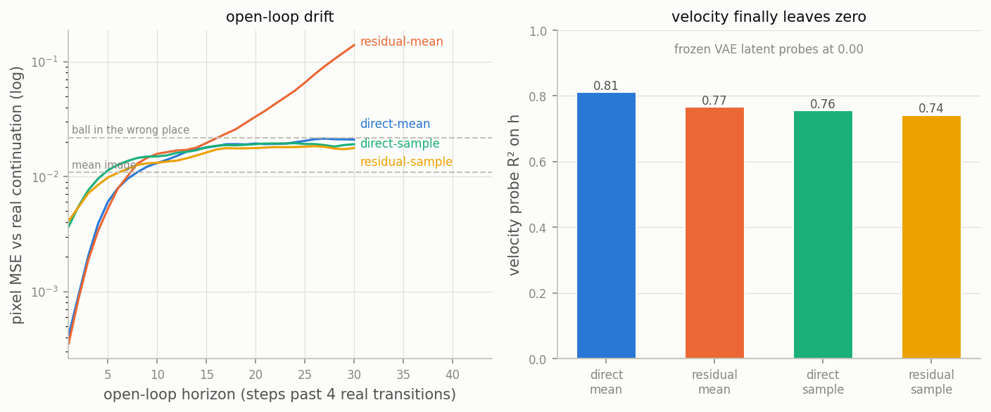
The zero moves: velocity 0.74 to 0.81
Velocity is linearly readable from every variant, against 0.00 from the encoder alone: the recurrence integrates motion, as the objective argument said it had to. The one-step number is startling for a model that has never seen a pixel, 0.00041 per pixel for direct-mean against a pipeline floor of 0.00027, so one step into the future costs about 50% more than repainting the present. Position reads 0.979 on where the raw latent managed 0.75; the box has the two mechanisms and the confound.
Why position jumps from 0.75 to 0.979, and the confound. A tangent; open if the position number bothers you.
Two mechanisms. Filtering: each frame's encoding is a noisy measurement of position, and a recurrence that has integrated many of them can average them, with estimation error falling roughly like , which is Kalman logic with the matrices learned rather than derived. Untangling: part 1 showed position present but curled in the latent, and a GRU that must use position to predict re-represents it in coordinates of its own, where 128 dimensions give it room to lie flat.
The caveat: a 128-dimensional vector flatters a linear probe relative to a 16-dimensional one on capacity alone, and this experiment cannot separate "better organized" from "more room to be organized in". That is why stays pinned at 128 for the RSSM, where the confound cancels.
The switch that detonates: residual-mean
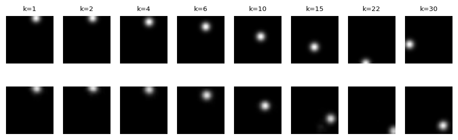
Residual prediction, trained on means, posts the best one-step error in the grid, and then explodes: 0.139 by horizon 30, more than six times above the hallucination ceiling.
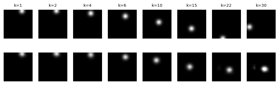
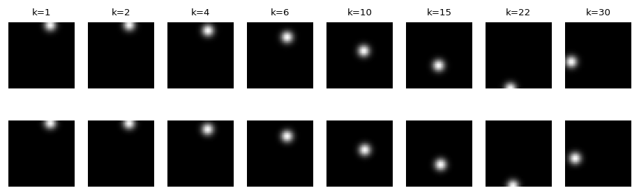
residual-mean rollout. Top row real, bottom row open loop. Through k=6 the rows are indistinguishable. By k=22 there is a vertical smear at the left edge that has never been a ball; by k=30 the blob is oversized, over-bright and still accompanied by its streak. This is what decoding an off-manifold latent looks like.The mechanism is the oldest one in numerical integration. Open loop, the residual model computes , a running sum; every step's small bias accumulates, nothing pulls the sum back toward latents the decoder has seen, and the state random-walks out of the data distribution. The direct model's update is , a fresh prediction of a plausible latent at every step, so errors saturate at "plausible but wrong" instead of compounding to "impossible".
Same objective, nearly identical teacher-forced scores (-20.7 against -21.6 NLL), completely different failure geometry. If you are going to roll a model out for 30 steps, measure it at 30 steps.
The switch that rescues it: train on samples
Training on samples costs you the short game and wins the long one.
The sample-trained runs are about 9 times worse at horizon 1, because the encoder's posterior noise is an error floor no model can beat. Both plateau below every mean-trained run by horizon 30, and the residual variant goes from 0.139 trained on means to 0.0177 trained on samples, best in the grid.
Figure 2 is the explanation. Teacher forcing trains the model on inputs from the real data distribution; open loop feeds it its own slightly-wrong outputs, which are inputs it has never seen, unless it trained on noisy latents, in which case "slightly wrong" has been in-distribution all along. Noise injection at training time buys robustness where open-loop rollouts spend it.
Dreamer (Hafner et al., 2019), the architecture in block 2, feeds its dynamics model samples rather than means. I had read that as an implementation detail for years; the grid says it is load-bearing.
Why the NLL column is not one leaderboard. Open before comparing -21.6 with +19.4.
The NLLs are only comparable within a latent source: sampled targets carry the posterior's irreducible entropy, so their likelihood floor sits about 40 nats above the mean-trained runs'. The mean-trained models are not "better" at -21.6 versus +19.4; they are being graded on an easier exam.
Where they all end up: one bounce of validity
Three of the four curves bend up toward the 0.022 line by to and flatten there (residual-mean keeps climbing). That plateau is the frozen recipe's ceiling, and it means about one bounce.
As the two-ball demo showed, a small error changes when and whether the next bounce happens, so the drift curve measures how long the model's timeline stays synchronized with ours. Block 2 asks how much of that ceiling is the frozenness itself.
2. Removing the seam: the RSSM
Result of this block: train the encoder and the dynamics against one loss and velocity goes to 0.96, reconstruction gets eight times better than the VAE's, and the model is still tracking a bounce at step 22. The architecture is the first six sections; the numbers start at "Results: frozen against joint".
Why delete the seam
Everything in block 1's results that could explain the ceiling is a property of the seam.
- The GRU spends capacity untangling and denoising a code that was shaped by reconstruction alone, which part 1 called the untangling tax.
- It cannot push information back into the encoder, so anything reconstruction discarded is gone for good.
Dreamer's answer is to delete the seam with a recurrent state-space model, the RSSM: one model, one loss, encoder trained by the prediction objective from the first gradient step.
Predict, then correct
Every filtering algorithm ever written has the same two beats: predict where the world should be, then correct that prediction with what you actually observe. A Kalman filter does it with matrices; an RSSM does it with a GRU and two small MLPs, and learns all of them.
The state comes in two pieces:
- , deterministic, 128 dimensions, carried by a GRU. This is memory. Given the past, it is a known quantity.
- , stochastic, 16 dimensions, resampled every step. This is everything the frame told you that memory could not have predicted.
Neither piece works alone. A purely deterministic state cannot represent uncertainty, and the random nudges make this world uncertain by construction; a purely stochastic state has to re-derive the whole past at every step through a sampling bottleneck. Splitting them routes predictable structure through , where it is cheap and exact, and reserves the noisy channel for what needs it.
The other half of the design is that the model gets asked the same question twice, once with the answer hidden and once with it visible. The prior must guess the stochastic state from memory alone. The posterior gets to look at the frame. Forcing the first to agree with the second is how dynamics get learned, and that forcing is a KL term.
The cell
A GRU core carries ; a prior head guesses from alone, a posterior head guesses it with the frame in hand, and a KL term between the two is the only thing connecting prediction to perception.
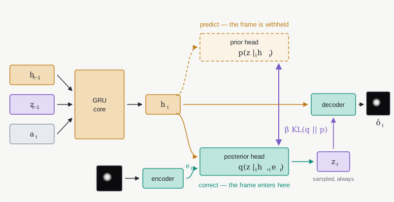
One step, given frame and action :
Block 1 paid for several of those choices:
- The decoder sees , the whole state. Reconstruction can lean on the deterministic path, which frees to carry only what could not predict; this is most of the explanation for the reconstruction result further down.
- is always a sample. The 2x2 grid showed that noisy inputs are what make a dynamics model robust to its own errors in open loop; what was a training trick there is how the architecture works here.
- has a floor of 0.1 on both heads, 100x the GRU's and the Dreamer default; like the GRU's floor it stops the model from driving and earning unbounded likelihood.
The encoder and decoder are the same conv stacks as part 1's VAE, is the same 128 as the GRU's, and the parameter counts are within 7% (box), so whatever is about to happen to the drift curve is not because I brought a bigger model.
Parameter count: RSSM 1.57M against the frozen pipeline's 1.47M. Open if you suspect a capacity mismatch.
The RSSM is 1.57M parameters. The frozen pipeline it replaces is 1.39M (VAE) plus 0.077M (GRU), so 1.47M. 7% apart.
The loss, and why this one did not collapse
This is part 1's ELBO with the sequence wrapped around it, except that the KL is against a learned prior where part 1 had , and that single difference is why the collapse that ate part 1's first run never happened here.
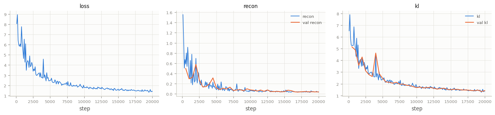
I trained with from step zero, warm-up knob untouched, and the KL settled at about 1.4 nats and stayed alive for 20k steps. What changed is the cost of "ignore the latent". Against a fixed prior the model can drive the KL to zero by matching and pay nothing; against a prior that chases the posterior, the KL is only large when the frame carried something the dynamics failed to predict, so carrying information is cheap from the first gradient step and there is no collapsed configuration to fall into.
The reward term is switched off until block 3; the plain ball has no reward.
The one trick: KL balancing
has two arguments and one gradient. Dreamer splits the gradient with stop-gradients while leaving the value alone, and no stabilization trick in the build carries more weight.
Left alone, the KL pulls both ways at once: the prior moves toward the posterior and the posterior gets dragged toward whatever the prior currently believes, which early in training is nothing useful, so that second pull is a regularizer toward ignorance.
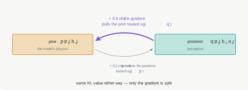
def kl_balanced(mu_q, sig_q, mu_p, sig_p, alpha: float = 0.8):
sg = jax.lax.stop_gradient
toward_prior = kl_gauss(sg(mu_q), sg(sig_q), mu_p, sig_p)
toward_post = kl_gauss(mu_q, sig_q, sg(mu_p), sg(sig_p))
return alpha * toward_prior + (1.0 - alpha) * toward_post
Four lines, easy to get backwards, so there is a test: at the posterior parameters receive zero KL gradient, checked with jax.grad. Write it, because a sign error here produces a model that trains, converges, and is wrong in a way no loss curve shows.
Training
One lax.scan with carry , pixels in, encoder inside the graph. Batches of 32 sequences (the GRU used 64); everything else, data, splits, 33 frames, warm-up 4, horizon 30, ridge probe, is pinned to the frozen run. One protocol difference: no loss mask on the first four transitions, because the posterior sees at every step, so early states are corrected rather than blind.
No learning-rate drop, no warm-up, no instability. I had lined up both levers in the design doc and used neither. RSSMs have a reputation for being touchy, and I record the non-event so that the next person's expectations are calibrated by something other than my anxiety.
The training step in code, which is also the imagination loop. Open if you are reimplementing, or want to see where block 3 swaps posterior for prior.
The per-sequence computation is the loop that generates imagination once you swap the posterior for the prior, which is what block 3 does:
def step(carry, xs):
h, z = carry
e_t, o_t, a_t, r_t, n_t = xs[:5]
h = model.apply(params, h, z, a_t, method=RSSM.core_step)
mu_p, sig_p = model.apply(params, h, method=RSSM.prior_dist)
mu_q, sig_q = model.apply(params, h, e_t, method=RSSM.post_dist)
z = mu_q + sig_q * n_t
o_hat = model.apply(params, h, z, method=RSSM.decode)
recon = ((o_hat - o_t) ** 2).sum(axis=(1, 2, 3)).mean()
klb = kl_balanced(mu_q, sig_q, mu_p, sig_p, config.alpha).mean()
...
Elided: the reward head's MSE term and the carry's return value. The full function is make_losses in train_rssm.py.
Results: frozen against joint
| metric | VAE latent | best frozen GRU () | joint RSSM () |
|---|---|---|---|
| velocity | 0.00 | 0.811 | 0.96 |
| position | 0.75 | 0.979 | 0.998 |
| drift @1 | n/a | 0.00035 | 0.000031 |
| drift @5 | n/a | 0.0053 | 0.00039 |
| drift @15 | n/a | 0.0162 | 0.0036 |
| drift @30 | n/a | 0.0177 | 0.0129 |
| reconstruction (summed) | 0.28 | inherits the VAE | 0.033 |
The middle column is generous on purpose: it takes the best of the four GRU variants per row, so the frozen recipe is represented by residual-mean on the short horizons, residual-sample on the long ones and direct-mean on the probes. RSSM probes are on alone, 128 dimensions, capacity-matched against the GRU's ; adding to the probe input buys about 0.003 more.
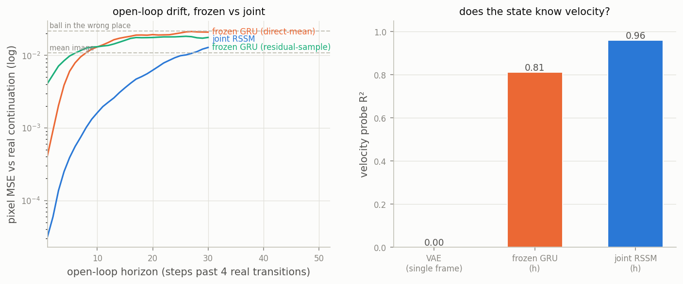
Subtract the decoders before reading the short-horizon gap
The joint curve enters 11 times better at one step and 13 times at five, and most of that is the decoder.
Each pipeline's drift is bounded below by its own reconstruction error, and the two floors are nothing alike: 0.00027 per pixel for the frozen stack, 0.000032 for the joint one. The frozen GRU's best one-step prediction is about 30% above its floor; the RSSM's is within rounding of its own, 0.000031 against 0.000032 (the floor decodes posterior samples and the drift rolls prior means, so the two are not strictly ordered). The faithful one-step statement is that predicting one step ahead costs the RSSM nothing measurable beyond redrawing the frame it already has, the frozen model pays about 30% extra, and the "11 times better" is that fact multiplied by a better decoder.
The long horizon is where the dynamics show
By the frozen model is 65 times above its floor and the joint one 400 times above its own, so the decoders have dropped out of the comparison.
There the RSSM reads 0.0129, just above the mean-image line at 0.011, and nowhere near the 0.022 ceiling where every frozen variant had parked. The joint model still retains information about the true trajectory at a horizon where the frozen recipe had decorrelated into "a perfect ball in an uncorrelated place".
Why it wins
The encoder stopped being an adversary.
In the frozen pipeline the GRU spent capacity untangling and denoising a code shaped by reconstruction alone. Here the encoder is shaped by the prediction loss from the start, so the latent arrives prediction-ready.
The cleanest evidence is the reconstruction row, the result I would have bet against: 0.033 summed error against the standalone VAE's 0.28, and the comparison is if anything unfair to the RSSM, whose figure decodes a posterior sample where the VAE's decodes the mean. I expected a reconstruction-versus-dynamics trade and got the opposite, because hands the decoder temporal context no single-frame encoder ever had: knowing where the ball was for the last thirty frames is extremely useful for drawing where it is now.
The KL is a task-complexity meter. Its equilibrium value is how many nats per frame the dynamics could not predict, and it costs nothing to log; the box has the numbers across the three tasks.
The KL as a difficulty meter across tasks (1.4, about 4, 5 to 6 nats), and why it is not comparable to part 1's 5.4. Open if you want to use the KL as a diagnostic.
For this environment the KL settles at about 1.4, roughly the injected action noise plus sub-pixel residue. Train the same architecture on the scene with a static goal ball in it and it settles near 4; let the goal move and it goes to 5 or 6. The number knew the difficulty ordering of the three tasks before I did.
Do not compare the 1.4 against part 1's 5.4 nats. That KL was against a fixed and priced the whole code; this one is against a learned prior and prices only the surprise.
Block 3 asks whether the model is good enough to train an agent inside.
3. Dreaming: an agent trained in imagination
Result of this block: an actor that never saw a real transition scores 0.88 on the follow task in the real environment, against baselines near 0.05, and its imagination underestimated the reward rather than gaming it.
The setup
A new version of the environment with a red goal ball rendered into the pixels, and a policy trained on nothing but the world model's own imagined rollouts.
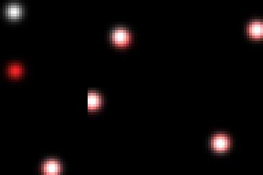
The goal has to be in the pixels because the reward depends on it. The observation goes RGB, the reward is a Gaussian kernel on the agent-to-goal distance, and one knob covers two tasks: the goal either sits still (hover) or cruises and bounces at half the agent's speed cap (follow).
The recipe is offline Dreamer. Freeze the world model, then train an actor and a critic only on imagined rollouts:
- Start from real posterior states filtered out of the replay data.
- Roll the prior forward 15 steps under the actor, with .
- Read rewards from the reward head and score with TD(): , with .
- The critic regresses onto ; the actor maximizes directly.
Because every piece is reparameterized, Gaussian latents, tanh-Gaussian actions and a differentiable reward head, the value gradient flows through the dynamics themselves: no REINFORCE, no target network, no environment interaction. The policy improves by backpropagating through its own imagination.
Results
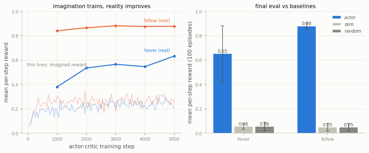
Evaluated in the real environment over 100 fresh episodes, the actor scores 0.65 on hover and 0.88 on follow, against baselines near 0.05.
| task | actor | zero | random | actor std |
|---|---|---|---|---|
| hover | 0.652 | 0.055 | 0.055 | 0.228 |
| follow | 0.879 | 0.048 | 0.049 | 0.025 |
What matters more than the scores
The imagination was pessimistic, not exploitative. I built the left panel of Figure 11 expecting to catch the actor conning its own reward head, the classic model-based failure. The opposite happened: imagined reward sits near 0.2 while real reward climbs past 0.8. The cause is horizon bias. Imagination only sees 15-step windows starting from random replay states, most of them far from the goal, so it mostly measures transit time; real 200-step episodes let the agent park on the goal and collect. Imagined return is a local-improvement signal, and episode return is a different quantity.
The harder task produced the better policy, because it produced the better world model. Follow beats hover 0.879 to 0.652, and the standard deviations are the tell: 0.025 against 0.228. The hover world model overfit its 400 static goal positions, the first train/validation gap of the project, so on some episodes it mislocates the target and the actor inherits the error. The follow model never had that option: 400 goal trajectories forced it to track, and it probes goal position at 0.99. Its actor locks on every single episode.
The policy is a mirror held up to the world model. Every flaw transfers.
One more probe that lied: the hover goal probe read 0.12. Open if you use probes on static targets.
One more entry for the file part 1 opened on probes lying in specific ways: the hover model's goal probe read 0.12, which looks damning until you notice that a static goal means the probe's fit set contains 25 effectively distinct target values dressed up as thousands of rows. Ridge memorizes 25 points in 128 dimensions and whiffs on the unseen 25. A probe needs variance in its target within its fit distribution, or it measures nothing.
Where this breaks
- One seed, one environment, 32x32 pixels. Every number is a single run. I would defend the 0.96-against-0.81 velocity gap and the factor-of-six divergence; the 0.998-against-0.979 position gap and the 0.811-to-0.766 spread across the GRUs, I would not.
- None of the four GRUs was tuned individually. A residual model with its own gradient clipping or a lower learning rate might not detonate; what I showed is that the default recipe does.
- The objective is reconstruction. On a ball in an empty box, what you need to draw is what you need to predict; add a distractor background, waving trees or TV static, and reconstruction spends its capacity on the irrelevant pixels because they occupy most of the image. That is the case for reconstruction-free objectives, and I plan a distractor-background version to make it visible.
- Continuous Gaussian latents. DreamerV2 (2021) and V3 (2023) use categorical latents with straight-through gradients, which are better at multimodal futures. For this world the Gaussian is fine, but "fine on a bouncing ball" is a weak claim about anything else.
- Capacity-matched rather than compute-matched, and the open-loop wall moved rather than vanishing. The RSSM does far more work per step (an encoder and decoder inside a 33-step scan, against a GRU over precomputed latents), and what that bought is the mean-image crossing moving from to plus an order of magnitude in error short of it: large practically, the same kind of thing. Both models eventually lose the timeline, which is what a stochastic environment does to open-loop prediction, and if wall-clock is your constraint the frozen recipe is cheaper and debugs in two independent phases.
Try it yourself: commands and four exercises. Open if you want to run it.
Same hardware and versions as part 1: RTX 5070 Ti under WSL2, JAX 0.10.1, Flax 0.12.7, Optax 0.2.8; everything runs on CPU too, slower.
uv run make-data
uv run train-gru --predict direct --latent-source mean
uv run train-rssm --run-name base
uv run make-data --task follow
uv run train-rssm --data data/ball_follow.npz --run-name follow
uv run train-ac --wm-run runs/rssm/follow --data data/ball_follow.npz \
--goal-speed 1.0 --run-name follow
- Predict before you measure. Before running the
residual-meanvariant, write down what you expect its horizon-30 drift to be. Then look. Nothing else in this project produced a bigger gap between my prediction and the measurement. - Break KL balancing on purpose. Train the RSSM with
--alpha 0.5and--alpha 1.0. At 1.0 the posterior gets no KL gradient at all. Predict what that does to the KL curve and to the drift before you look. - Take the prior's uncertainty seriously. The drift curves above roll prior means. Roll prior samples instead and plot both. The sampled curve sits slightly higher, and the gap is the model's own uncertainty rendered in pixels, a free calibration check on whether the it reports is honest.
- Kill the action channel. Retrain the GRU with the action input zeroed. The ball's motion is mostly ballistic, so the drift curve should barely move at short horizons and degrade at long ones, where accumulated nudges matter. If it doesn't degrade at all, check that the nudges in your dataset are actually reaching the velocity.
What moved the zero
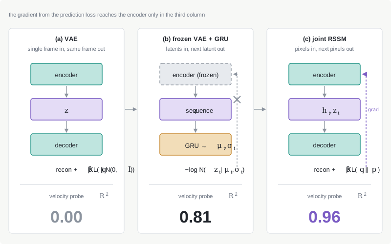
A representation is shaped by the loss that reaches it. Train an encoder on reconstruction and you get a code that knows what a frame looks like. Train it on prediction and you get a code that knows what the world does next, and, as it turns out, one that also knows better what the frame looks like.
Next stop is the environment this was all rehearsal for: the same recipe, pointed at DOOM's take_cover, where nobody hands you the true state and every measurement in this series has to be earned a different way.