August 11, 2026
World Models From Scratch, Part 1: A Ball, a VAE, and a Number That Would Not Move
A VAE can reconstruct every frame perfectly and still know nothing about how the world moves. A toy environment where I know the ground truth, a linear probe that catches the latent out, a collapse that converged to exactly 11.17, and a dead model that scored 0.74.
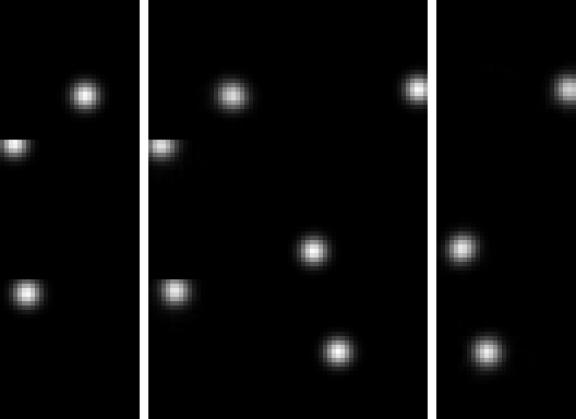
A model can reconstruct every frame you show it, pixel for pixel, and still know nothing about how the world moves. I found that easy to nod along to and hard to believe until it happened in my own code, on a dataset small enough to hold in my head. So this series builds the whole thing from scratch, on a world I wrote: a VAE, then Ha and Schmidhuber's frozen-encoder recurrent model from World Models (2018), then the RSSM from Dreamer (Hafner et al., 2019). Same dataset, same evaluation, one number decides who wins.
What you need: convolutional networks, maximum likelihood, and enough JAX to read a lax.scan. Code is at github.com/RetamalVictor/world-models; every number below comes from a seeded run in that repo.
The instrument: a linear probe on a world I can see inside
*Every model in this series is graded on one question, did the latent learn the dynamics?, and the only way to answer it is to own the ground truth.*
On Atari or DOOM you cannot. You can look at imagined rollouts and say "hm, plausible", but nobody will tell you where the ball was actually going, because the ground truth is inside the emulator and the emulator does not export it. So I wrote a simulator that does.
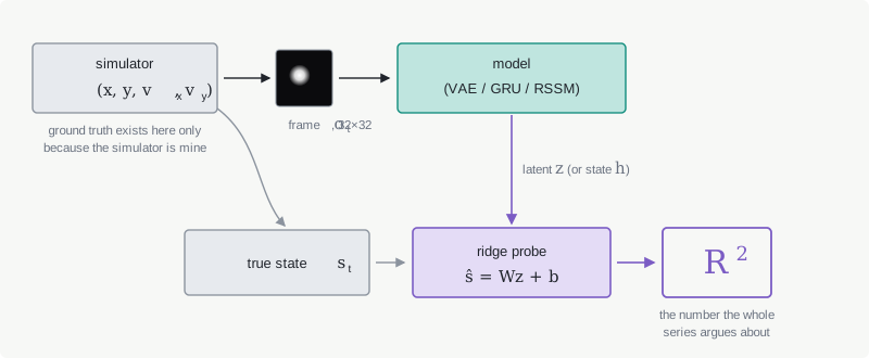
Definition (the probe). Fit ridge regression from a model's state to a ground-truth quantity on one set of held-out episodes, and report on a second, disjoint set:
One is perfect, zero is "no better than predicting the mean of ", negative is worse than a constant. The whole probe is four lines, deliberately not sklearn, so you can see all of it:
def ridge_fit(X, y, lam: float = 1e-3):
"""Ridge regression with intercept. X: (N, D), y: (N, K) -> (w, b)."""
x_mean = X.mean(axis=0)
y_mean = y.mean(axis=0)
Xc = X - x_mean
yc = y - y_mean
d = X.shape[1]
w = jnp.linalg.solve(Xc.T @ Xc + lam * jnp.eye(d), Xc.T @ yc)
b = y_mean - x_mean @ w
return w, b
Both rules baked into that function bite later.
- The probe is linear. A nonlinear probe with enough capacity recovers position from almost anything, including a randomly initialized network, and measures the probe rather than the model.
- It is fit on one set of episodes and scored on another. Frames inside one episode are near-duplicates of their neighbors, so a frame-level split leaks the test set into training through a wall of correlated pixels.
The world: a ball in a box
State is , the action is a nudge added to the velocity, and the observation is a 32x32 grayscale image with a Gaussian blob centered on the ball. Everything hard happens at the wall bounces.
Here it is running: the same forty lines of physics and rendering the training data came from, in TypeScript, in your browser.
Pause, then say which way the ball is moving. The renderer is a function of position alone, so the frame cannot tell you.
Watch the wall bounces. Between them the motion is a linear extrapolation any model can do; at a bounce, a half-pixel error in position decides whether the reflection happens this frame or the next, and two trajectories that agreed perfectly diverge at full speed. Then pause it on a single frame. That is what a VAE gets, and the question this post ends on is whether anything in that picture says which way the ball is moving.
The physics fits on one screen:
vx = state.vx + ax
vy = state.vy + ay
speed = jnp.sqrt(vx ** 2 + vy ** 2)
scale = jnp.where(speed > params.max_speed, params.max_speed / speed, 1.0)
vx = vx * scale
vy = vy * scale
x = state.x + vx * params.dt
y = state.y + vy * params.dt
x, vx = _reflect(x, vx, jnp.float32(params.img_w))
y, vy = _reflect(y, vy, jnp.float32(params.img_h))
The choices in there that matter downstream:
- The blob is Gaussian. A hard-edged sprite quantizes position to the pixel grid; a Gaussian blob shifts intensity smoothly, so the image encodes sub-pixel position and the reconstruction loss has a gradient everywhere. That is why the position probe can score above 0.9 in principle.
- Walls reflect rather than clamp. Velocity flips sign and the overshoot folds back, so energy is conserved and there is something worth modeling. One reflection per axis per step is enough only because
max_speed(2.0) is far below the box size (32). - The true state rides along in
info. Everystepreturnstrue_x,true_y,true_vx,true_vy, which is the environment's whole reason to exist.
The dataset
One fixed file, generated once, shared by all three models, split at the episode level, and 98% black.
uv run make-data # 500 episodes x 200 steps, random_nudge_policy(0.3), seed 0
500 episodes of 200 steps, frames as uint8 (about 100 MB), actions and true state as float32. Episodes 0 to 399 train, 400 to 449 validate, 450 to 499 test. The probe fits on episodes 450 to 474 and scores on 475 to 499, for every model in this series, so the numbers stay comparable by construction.
statistic (data/ball.stats.json) |
value |
|---|---|
| pixel mean | 0.0221 |
| pixel std | 0.1045 |
The frames are 98% black. The std sets the value the first run's loss will converge to, below; the blackness is why that run finds the collapse so comfortable.
The VAE: a noisy channel with a price per nat
The picture to keep: the encoder is buying bandwidth, and is the price per nat.
An autoencoder squeezes an image through a bottleneck and asks for it back. Whatever survives the squeeze is what the model considered worth keeping. Stop there and you get a code that works but has no particular shape, because nothing in the objective cares how the 16 numbers are arranged.
A variational autoencoder adds one thing: the bottleneck is a noisy channel. The encoder emits a distribution over codes, and the decoder receives a sample from it. Now sloppiness has a price. If two frames map to overlapping distributions, the decoder cannot tell them apart; if the encoder wants to be certain, it pays, and the currency is the KL term.
The loss, as implemented:
One thing about that the derivation in the box makes obvious and the code hides: is a claim about the data. It equals , the decoder's assumed observation noise, so asserts per pixel on frames whose own standard deviation is 0.1045. You are telling the model the image is mostly noise. Remember that when the first run collapses.
Where the loss comes from: the ELBO, and why β = 2σ². Derivation; skip unless you want to re-derive the loss.
We want to maximize for a latent-variable model , which is intractable. Introduce any distribution and apply Jensen's inequality:
The right-hand side is the evidence lower bound, ELBO from here on. The gap between the two sides is , so the bound is tight when the encoder matches the true posterior. Maximizing the ELBO does two jobs at once: it pushes up the likelihood and it drags toward the posterior it can never compute.
Turning that into code takes a few concrete choices:
- The prior is with . The ball has four true degrees of freedom; 16 leaves headroom without letting the probe flatter the model.
- The encoder is a diagonal Gaussian, , so the KL has a closed form.
- The decoder is a Gaussian with fixed variance, which makes the reconstruction term a plain squared error: .
Minimizing the negative ELBO therefore means minimizing . Multiply through by , which changes nothing about where the minimum is, and you get the loss that is actually implemented, with .
Once you tune freely you have left the ELBO and entered -VAE territory, where the KL is a disentanglement pressure rather than a likelihood term. That turns out to be a feature, and the probe section below is where it pays off.
The reparameterization trick, and the one line of Flax that does it. Skip if you have seen it.
We need , and the parameters sit inside the distribution we are sampling from. Write the sample as a deterministic function of the parameters and a fixed noise source:
Now the randomness is an input, the path from to is differentiable, and a single sample gives a low-variance gradient. In Flax it is one line, which rather undersells it:
def __call__(self, x, key):
mu, logvar = self.encoder(x)
std = jnp.exp(0.5 * logvar)
z = mu + std * jax.random.normal(key, mu.shape) # reparameterization
recon = self.decoder(z)
return recon, mu, logvar
The network
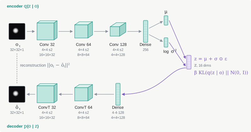
Three stride-2 convolutions take 32x32 down to 4x4, a dense layer to 256, then heads for and ; the decoder mirrors it. 20k steps take about two minutes on the GPU, which is the real reason a toy environment is worth building. You can afford to be wrong six times before lunch.
Architecture and training details: activations, why the losses are sums, optimizer settings. Open if you are reimplementing.
Channels widen 32 to 64 to 128 across the three convolutions. SiLU activations throughout; the final layer is linear, because its output is a Gaussian mean. Both loss terms are sums, reconstruction over the 1024 pixels and KL over the 16 latent dimensions, averaged over the batch. Summing rather than averaging is what keeps interpretable as a price.
Training: Adam at , gradients clipped at global norm 1.0, batch 128, 20k steps.
Three runs, one of them dead
I ran the textbook configuration first, constant from step zero, and it died. Two variants lived.
| run | schedule | KL (nats) | val recon | position | velocity |
|---|---|---|---|---|---|
base |
1.0 from step 0 | 0.00 | 11.17 | 0.74 | -0.005 |
beta01 |
0.1 fixed | ~9.6 | 0.06 | 0.35 | -0.013 |
warmup5k |
1.0, 5k linear warm-up | ~5.4 | 0.28 | 0.75 | -0.013 |
Units, because they bite for the rest of the series: reconstruction is squared error summed over all 1024 pixels and averaged over the batch, decoding the posterior mean. KL is in nats, summed over the 16 latent dimensions; a nat is a bit taken in natural log, about 1.44 bits. Part 2 works in per-pixel error instead, the same quantity divided by 1024.
base: posterior collapse, and why 11.17 is not a random number
The KL hit zero inside the first thousand steps and never came back, and the reconstruction error converged to the cost of painting the mean image.
A zero KL sounds like efficiency, and it is fatal. Against a unit Gaussian prior the KL vanishes in one configuration only:
The posterior is the same distribution for every frame; whatever the encoder computes on its way there, none of it survives. And the expected KL upper-bounds the mutual information between the frame and the sampled latent,
so a KL of zero nats means carries zero information about its frame. The decoder is being handed noise, and the best thing any function of pure noise can do under squared error is emit a constant.
Which constant? The reconstruction number sat at 11.17 for 20k steps, and 11.17 is a very particular value:
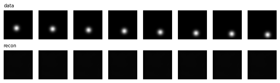
The loss was not stuck. It had converged, to the best answer available to a decoder that ignores its input, and at from step zero the exit is too expensive to find, because every nat the encoder buys costs a full unit of squared error before it has a decoder good enough to spend it on.
warmup5k: ramp the price
Keep as the target, ramp it linearly over the first 5k steps, and the collapse never happens.
uv run train-vae --run-name warmup5k --beta 1.0 --beta-warmup-steps 5000
Early on, information is nearly free, so the decoder learns to use the latent while nobody is charging for it. By the time the full price kicks in, "ignore the latent" is no longer the optimum it was at initialization.
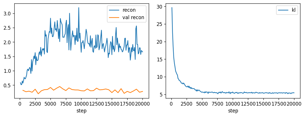
warmup5k. Right panel: the KL falls from about 30 nats to about 5.4 as the ramp ends and stays there for 15,000 more steps. No re-collapse; the model has found the amount of information about a frame that is worth paying full price for.Gotcha in the left panel: why training reconstruction sits above validation. Open if Fig 4 looks like a broken generalization gap to you.
Training reconstruction (about 1.7) sits above validation (about 0.28), which looks like the world's most broken generalization gap. It isn't. The training curve decodes a sample ; the validation curve decodes the posterior mean. The gap is the sampling noise the model is trained to tolerate, two different quantities with the same name on the same axis.
What a nat buys: the per-nat table, and why 5.4 nats is slightly-under-pixel precision. An aside; open for the rate-distortion reading.
The model minimizes , so a nat is worth buying only if it saves at least units of squared error, and the total saving available is bounded by 11.17, the cost of knowing nothing. Cheap nats get spent freely; expensive nats get spent carefully.
| run | nats bought | recon (summed) | error saved | per nat | |
|---|---|---|---|---|---|
beta01 |
0.1 | 9.6 | 0.06 | 11.11 | 1.16 |
warmup5k |
1.0 | 5.4 | 0.28 | 10.89 | 2.02 |
The 5.4-nat figure has a physical reading. Pixel-precise position in a 32x32 box costs about nats, so 5.4 nats is position at slightly-under-pixel precision, which is what the reconstructions look like.
These are two separate runs rather than two points on one rate-distortion frontier, so read "per nat" as an average. Measuring the real frontier means sweeping ; that is exercise 2 at the end.
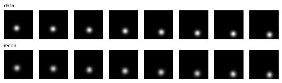
warmup5k, rebuilt from 16 numbers each. Every ball lands where it should, slightly softer than the original: the sub-pixel precision the KL budget could not afford.What that grid cannot show is the one thing this project is about, holding on to something across time, because every frame is encoded independently. Here is the clip from the top of the post again, with the stakes attached:
warmup5k on the right. 200 frames, each one encoded with no knowledge of the last.It tracks perfectly, and it tracks statelessly. A model that follows a ball this well for 200 frames is about to score zero on the one question that needs two of them.
Better reconstruction, worse probe
beta01 reconstructs better than warmup5k (0.06 against 0.28 summed error) and probes half as well (0.35 against 0.75), on the same architecture, data and step count.
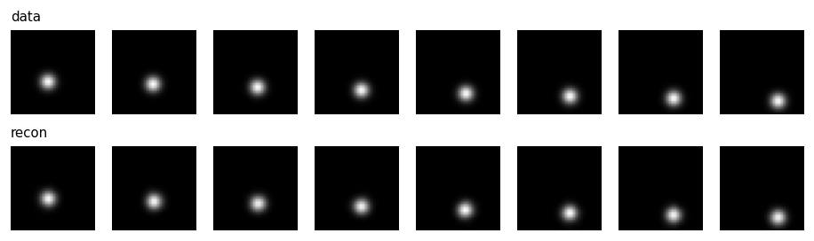
beta01 model reconstructing held-out frames. Near pixel-perfect: the position is in those 16 numbers, and the decoder is drawing it. The position probe should be a formality.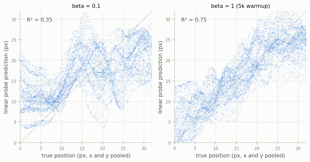
Reconstruction can never settle this question. Take any trained VAE with encoder and decoder , and any smooth invertible map on the latent space: the pair reconstructs identically, because the warp and the unwarp cancel before the decoder draws a pixel. A linear probe is precisely a measurement of the coordinate system reconstruction is blind to, since it lives or dies on whether is an affine function of , and almost any destroys that while leaving reconstruction untouched.
"The information is present" is invariant under reparameterization. "The information is linearly accessible" is not.
So what can prefer straight codes? The only other term in the loss. Against a factorized prior the KL decomposes per coordinate:
That expression has opinions. It charges each axis separately for deviating from , so among all the reconstruction-equivalent codes it prefers the zero-centered, unit-scaled, axis-factorized ones, and is the volume knob on that preference. This is the -VAE result from Higgins et al. (2017). I knew it as a citation before I watched it double a number I cared about in a two-minute run.
Part 2 is why this matters: it bolts a recurrent model onto these 16 numbers with the encoder frozen. A GRU can in principle learn and straighten the code before predicting, but "first untangle, then predict" is a tax paid in capacity and data, and 0.75 is the number that tax gets measured against.
The probe can lie: a dead model scored 0.74
The collapsed base model, KL pinned at zero, decoder painting black squares, reads 0.74 on the position probe. The healthy warmup5k reads 0.75.
That should be impossible: the base section's inequality bounds at zero when KL , so the latent contains nothing. But the bound governs the sampled latent , the thing the decoder eats, and the probe never touches . It reads , a deterministic function of the input, and appears in no inequality anywhere in the ELBO.
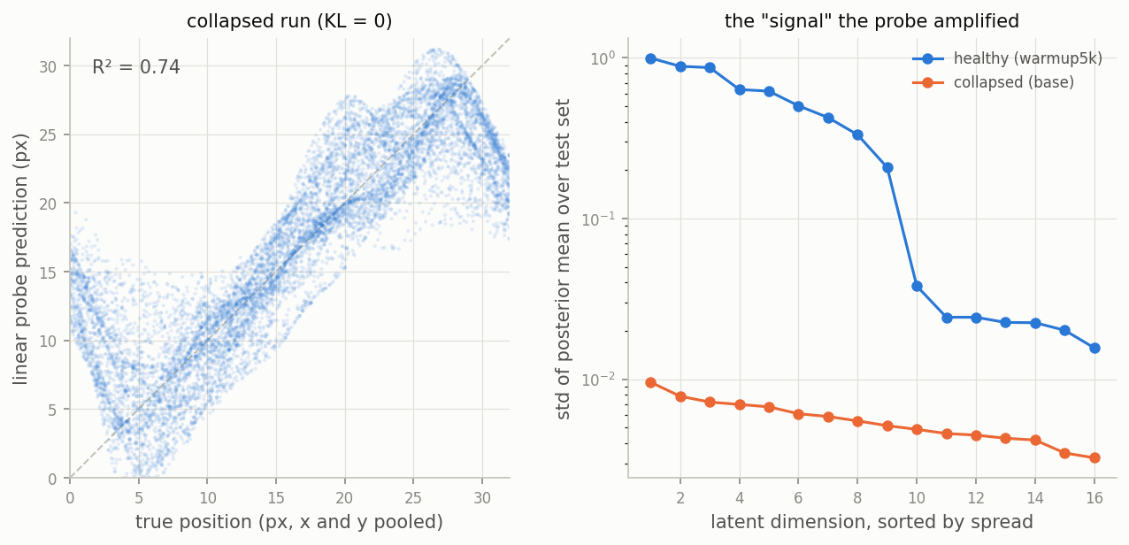
How the 0.74 happens:
- never went to zero, because it didn't have to. At and the per-dimension KL cost is about nats, so "KL = 0.000" in my logs was never zero, only cheap.
- Ridge regression does not care about magnitude. Rescale a code by any and the fit becomes with unchanged, so the probe multiplied microscopic wiggles by 200 and read position straight back out.
- The model itself cannot use that signal. The decoder sees at an SNR of , while the probe reads directly at infinite SNR; same encoder, two channels, both measurements correct.
There is an older result this rhymes with: linear probes on randomly initialized convolutional networks beat chance comfortably, so if architecture alone can carry a probe, a probe alone cannot certify learning.
The rule this bought, which part 2 obeys throughout:
A probe never travels alone. Report it with the KL (how much the sampled latent could carry) and the reconstruction error (whether the model cashes it in). Any one of the three can flatter a broken model; it is much harder for all three to coordinate on the same lie.
The zero this post existed to produce
Velocity probe, all three runs, healthy and dead: .
This is a property of the renderer: the observation is _render(x, y, params), a function of position alone, so and no single-frame encoder, at any capacity, with any , trained for any number of steps, can do better than chance.
Velocity lives in the difference between frames, and a VAE never sees two frames at once.
That zero is the baseline. Everything part 2 does is an attempt to move it, and the fair way to grade a dynamics model is to ask what it recovers that a single frame provably cannot contain.
Where this breaks
- One seed. Every number is a single run at seed 0; the gap between 0.35 and 0.75 is large enough to believe, and the gap between 0.74 and 0.75 is not a measurement of anything, which is rather the point.
- One environment, and an easy one. Static background, one object, no occlusion. The 98%-black statistic that made collapse so easy is a property of this dataset; on a busier scene "paint the mean image" is a much worse optimum and may behave completely differently.
- The latent size is a choice. At 16 dimensions the model uses about nine. At 4 it would be forced to be efficient; at 64 the probe would look better only because a linear map from 64 dimensions has more room to fit, which is why part 2 holds fixed across models.
- The position expectation was wrong and I revised it. My design doc said position . It landed at 0.75. The honest reading is that 0.75 is what buys at this latent size, but I wrote the criterion first and missed it, and that belongs in the record rather than in a quietly edited design doc.
Try it yourself: commands, hardware and versions, and three exercises. Open if you want to run it.
Everything below runs on CPU, slower but identical to a few decimals. The GPU runs in this post were an RTX 5070 Ti under WSL2, on JAX 0.10.1, Flax 0.12.7 and Optax 0.2.8; each run's config.json records the backend it used.
uv sync
uv run make-data
uv run train-vae --run-name warmup5k --beta 1.0 --beta-warmup-steps 5000
Artifacts land in runs/vae/warmup5k/: config.json, metrics.jsonl, reconstruction and prior-sample grids, and probe.json with the numbers. The environment API is gymnax-shaped, reset(key, params) and step(key, state, action, params) as pure functions with a static NamedTuple of params, which is what lets part 3 swap in ViZDoom without touching the model code.
- Reproduce the collapse. Run
train-vae --run-name basewith the default constant and watchreconinmetrics.jsonlflatten. Predict the value it flattens at before you look, from the pixel std indata/ball.stats.json. - Move the price. Sweep over 0.03, 0.1, 0.3, 1 and 3, and plot KL against reconstruction error. That plot is the rate-distortion frontier I admitted to not measuring above. Where does the position probe peak, and is it at the same that reconstructs best?
- Break the probe on purpose. Encode the test set, apply an invertible nonlinear warp to the latents, say elementwise, and re-run the probe. Reconstruction through the inverse is unchanged; watch fall. This is the reparameterization argument, made experimental.
Next: part 2 freezes this encoder, bolts a GRU onto its latents in the World Models (2018) style, and asks the zero to move. It moves to 0.81, and then to 0.96 once the encoder is allowed to learn from the prediction loss too. One of the four models along the way detonates.